V. Growth and Inequality

GROWTH AND INEQUALITY

[W]hatever disadvantage or detriment the introduction and use of new and improved instrumentalities or methods of production and distribution may temporarily entail on individuals or classes, the ultimate result is always an almost immeasurable degree of increased good to mankind in general. [However] That many of the features of the situation are, when considered by themselves, disagreeable and even appalling, can not be denied.

DAVID A. WELLS

REGIONAL DISPARITIES IN DEVELOPMENT

Generalizations concerning the entire United States must often be qualified to take into account substantial differences among regions; such was the case in our discussions of population growth, urbanization, and agricultural development. Personal income per capita, a crude measure of the average level of material well-being, also differed markedly in the various parts of the nation. Among contemporaries these differences sometimes gave rise to political antagonism, and “sectional” issues play a large part in American political history. In 1880, the first year within the post-Civil War era for which state income data are available, estimated personal income per capita varied from a low of $46 in North Carolina to a high of $318 in Nevada. Southern states generally had income levels of about half the national average; some Western states had income levels more than twice the national average; and other states varied between these extremes (Table 5.1).

TABLE 5.1
REGIONAL PERSONAL INCOME PER CAPITA RELATIVE TO THE NATIONAL AVERAGE (NATIONAL AVERAGE = 100)

Regions	1880	1900	1920
Northeast	141	137	132
New England	141	134	124
Middle Atlantic	141	139	134
North Central	98	103	100
East North Central	102	106	108
West North Central	90	97	87
South	51	51	62
South Atlantic	45	45	59
East South Central	51	49	52
West South Central	60	61	72
West	190	154	122
Mountain	168	139	100
Pacific	204	163	135

SOURCE. Richard A. Easterlin, “Regional Income Trends, 1840–1950,” in Seymour E. Harris, Ed., American Economic History (New York: McGraw-Hill, 1961), p. 528. Regions are defined as in Table 2.8. The relative income of 163 for the West in 1900, which is given in the above source, is in error. The figure given here, 154, is computed from data shown in Richard A. Easterlin, “Interregional Differences in Per Capita Income, Population, and Total Income, 1840–1950,” in National Bureau of Economic Research, Conference on Research in Income and Wealth, Trends in the American Economy in the Nineteenth Century (Princeton, N. J.: Princeton University, 1960), p. 137.

Southern income levels remained substantially below those elsewhere throughout the post-Civil War era, but scholars have too often exaggerated the problems of Southern development. Statistics themselves—it would be more accurate to say naively interpreted statistics—are partly to blame for a fascination with Southern “backwardness” and “stagnation.” Money wage levels, for example, were typically lower in the South than elsewhere; but because the prices of consumer goods were also typically lower, the gap between real wages in the South and elsewhere was less than simple comparisons of money wage figures would indicate. Correction for the relatively high prices of the Far West, it might be added, would substantially reduce the relative incomes of that area. Even when we make such corrections, however, it remains true that Southern earnings on the average fell below those elsewhere. No special theory of “Southern backwardness” is required to explain this differential; indeed, it can be explained by a general theory that accounts for differences of income levels among all the regions.

Economic theory asserts that output (or income) per worker differs among regions because of differences in the amounts of material, human, and intellectual capital—inputs that are generally highly correlated with one another—each worker has to assist him in production. As we saw when investigating agricultural output per worker in the various regions, the crude and indirect evidence that exists is consistent with this hypothesis. Although we lack the kind of data that would permit a direct test of the more general hypothesis concerning regional income differentials, a variety of indirect evidence is consistent with it. One study found that among the states in 1919, wages per worker and material capital per worker in manufacturing were significantly related.¹ Many studies of more recent periods have discovered such a significant relation, which causes us to suspect that the relation also existed in the earlier period. We emphasize again, however, that such evidence is consistent with the hypothesis only under the assumption that the three kinds of capital accumulation are highly correlated.

Investment in formal education was closely related to the level of income per capita. Notably, the cluster of states in the lower left corner of Figure 5.1, a position indicating both relatively low investment in formal education and relatively low income, consists of the 11 states of the Confederacy plus Kentucky and West Virginia; the lowest ranking non-Southern state exceeds the highest ranking Southern state in both dimensions of the figure. The relation also obtained among the non-Southern states, with the exception of two frontier mining states, Nevada and Colorado, for which the divergencies have an obvious explanation. Of course, the correlation portrayed in the figure does nothing to establish the direction of causality, but it is consistent with the hypothesis that relatively small investments in human capital contributed toward relatively low per capita incomes among the various states.

Between 1880 and 1900, income per capita increased as rapidly in the South as in the non-South, while Western incomes grew substantially slower and Northeastern incomes slightly slower than the national average (Table 5.1). Contrary to assertions of Southern “stagnation” in the post-Civil War era, the South did not lag behind the rest of the nation after 1880. Of course, even though its rate of growth was equal to the national average, the absolute difference between Southern and non-Southern income levels became wider. Perhaps this is the gap that historians and other observers have had in mind when discussing the increasing “backwardness” of the South. Regional groupings obscure substantial differences among the individual states, but the dispersion of the states around the national average level of income did become somewhat smaller during the two decades after 1880. Between the turn of the century and 1920 the South made large gains, while the Northeast and the West again sustained losses relative to the national average. Overall, the four decades after 1880 witnessed a relative narrowing of regional differences in personal income per capita.

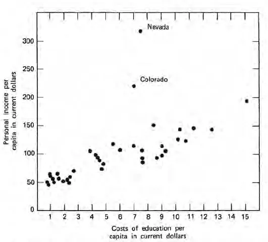
Figure 5.1 Relation between income and investment in formal education, by states, 1880. Source: Lewis C. Solmon, “Estimates of the Costs of Schooling in 1880 and 1890,” Explorations in Economic History, VII (Supplement: 1970), 534.

How can this narrowing be explained? A theory to answer this question is a simple extension of the theory employed to explain regional differences at a point in time. At any given time in the post-Civil War era the resource endowment of any region differed from that of other regions. For example, the West possessed relatively large quantities of land, the Northeast relatively large quantities of all kinds of capital except land, and the South relatively large quantities of unskilled labor. The resource that was relatively most abundant in a region commanded a relatively low rate of return. For instance, unskilled laborers in Alabama, where they were relatively abundant, earned a lower real wage than they did in California, where they were relatively scarce. Resource owners sought to obtain higher returns by moving their resources—whether labor or some form of capital—to areas characterized by a relative scarcity of that resource. Workers migrated to places where they could obtain higher real wages, and capitalists sought to invest in areas promising the highest rate of return, as we have already seen in the discussion of farm mortgage lending.² If underlying economic conditions had remained unchanged, such movements would eventually have resulted in an approximate equalization of returns among all regions for each kind of resource. But of course the world did not stand still. Before a complete adjustment had been made, new changes occurred in demand and technology, upsetting the old pattern of adjustment. In practice, therefore, the interregional transfer of resources produced only a tendency toward equalization of returns, never an actual realization of equality. Moreover, some of the adjustments occurred at a snail’s pace, so divergencies persisted throughout the period, especially when the causes of the original divergencies were self-reinforcing. The same differentials among returns that gave rise to interregional migration of resources also encouraged individuals within each of the regions to accumulate that form of capital being attracted from other areas. Together the accumulation of capital within regions and the transfer of resources among regions produced the tendency toward equalization.

What we know about the movement of resources in the post-Civil War era is broadly consistent with the hypothesis just sketched. Net in-migration relative to population was largest in the West and substantially lower in the Northeast and Great Lakes regions; and in the South the number of out-migrants exceeded the number of in-migrants in every decade of the period. Eastern capitalists did transfer their resources to the South and the West more frequently than the reverse occurred. With workers moving into areas of relative labor scarcity and capital into areas of relative capital scarcity, the ratio of capital to labor drew closer to equality among the regions, and a narrowing of interregional income differentials was the consequence. That differences remained is attributable to deficiencies of information about opportunities elsewhere, to costs of transferring resources, to difficulties in borrowing to finance the transfer, and to continuing disturbances in the economy that altered the distribution of opportunities among the regions and changed the desirable pattern of adjustments.

It is curious that historians have often condemned the capital movements among regions as harmful to the areas receiving the capital. The distinguished historian of the South, C. Vann Woodward, for example, refers again and again to the “heedless exploitation of Southern resources and people by Northeastern capital.”³ This interpretation is simply wrong. Surely any reasonable definition of “exploitation”—though this value-laden word would be better abandoned than defined—requires that an “exploited” region be worse off than it would be if left “unexploited.” But the transfer of Northeastern resources into the South certainly did not make that region worse off; rather, the reverse was true. Even had the owners of the capital removed all their earnings from the region—which they did not—the South would still have benefited from the increased demand for local labor and materials, the expanded tax base, and all the benefits attributable to the new activities for which the owners could not charge—for example, the learning from experience gained by their employees. Interregional transfers of resources occurred through free contracting among the parties involved; that individuals voluntarily arranged the transfer suggests that each side considered the arrangement to its own advantage.

Underlying the claims of regional “exploitation” seem frequently to be the implicit assumptions that all regions “should” be equally industrialized and that while manufacturing is a Good Thing, agriculture and mining are activities fit only for slaves and other “exploited” people. Such views make no sense. The people of any region can maximize their incomes by pursuing the activities that make relatively intensive use of resources that are relatively abundant, and hence relatively cheap, in that region. To pursue other activities would be to sacrifice the benefits of specialization and trade. It is obvious that given the resource endowments of their regions, the advantage of Southerners and Westerners lay mainly in agriculture and other extractive industries, while Northeasterners stood to gain by concentrating on manufacturing and other nonagricultural activities. No one had to dictate these patterns of specialization, and no one did. The rate of return on the various activities attempted in the different regions provided a signal, informing entrepreneurs of the ways in which they, and therefore their regions, could obtain the highest possible incomes.

If we agree that interregional differences in income per capita resulted from differences in the capital/labor ratio and that during the 1880–1930 period the South actually gained on the rest of the nation, the really crucial question becomes: why was the capital/labor ratio relatively so low in the South in 1880? How could one region fall so far out of line with the others in an economy of mobile—though not costlessly mobile—resources? To answer this question requires a digression to consider the prewar economy.

Before the Civil War, slaves lacked property rights of any kind. Moreover, they were property, the most important form of Southern capital except land. In applying economic theory to predict the decisions of investors before the war, we must consider slaves in the same terms as machines, land, or inventories, simply as a form of capital. Under such circumstances economic theory predicts that the interregional flow of resources would tend to equalize only the incomes per capita of the free population of each region. And indeed the evidence is consistent with this prediction. Richard Easterlin found that in 1840, “if the slaves and their income (estimated at subsistence) are eliminated, one finds that the income of the white population in the South exceeded the national average and compared favorably with that of the Northeast.”⁴ Because Southern incomes grew somewhat more rapidly than the national average during the two decades before the Civil War, the level of Southern personal income per white capita exceeded the national average even more in 1860.⁵

The emancipation had two important effects. First, it destroyed part of the assets owned by the whites by outlawing their property rights in slaves; second, it added about four million persons to the Southern free population. Emancipation in no way affected the stock of real resources in the South; from a social point of view it destroyed nothing. In effect, it merely relabeled “machines” as “citizens” and gave them property rights to match their new status. (That the actual rights of blacks turned out to be more restricted than those of whites does not affect the present argument.) This change raises insurmountable problems of intertemporal comparison. To compare the level of income per free capita in 1860 with the same measure for a postwar year makes no sense; but neither does a comparison of incomes per capita of the total population when a third of that population consisted of “machines” at the first date. Per capita incomes at the two dates simply are not comparable in any meaningful sense. The emancipation in a single stroke increased the denominator of the fraction (income/free population) by transforming part of the capital stock into part of the population. Of course the level of income per free capita then dramatically declined, quite apart from the vast wartime destruction of Southern human and material capital. By a revolutionary restructuring of property rights the emancipation created a completely different set of feasible opportunities from the investor’s point of view, changing the slave owner’s valuable asset into the body of a new citizen. In this new legal framework investors, including now the freed-men, groped toward an adjustment, channeling their investments into those avenues—including migration—promising the highest rate of return. But we would hardly expect the achievement of a new equilibrium to occur immediately. The blow to the Southern asset structure was too disturbing for Southerners to adjust to quickly; in the economist’s jargon, the emancipation created a massive “portfolio disequilibrium.” In addition, postwar conditions did little to assist and much to retard a new adjustment.⁶ In retrospect, it is perhaps most remarkable that the Southern economy managed to rebound as quickly as it did.

A major implication of the preceding arguments deserves to be emphasized. The decline of Southern incomes below the national average is entirely attributable to the Civil War and its effects, and the region has been catching up ever since. The relative poverty of the South in the post-Civil War era—and indeed right up to the present day—is therefore entirely attributable to (1) the existence of the slave system and (2) the abolition of that system through destructive civil war and haphazard emancipation. Moralists might well hold Southerners accountable for the first, but hardly for the second. How ironic that the Great Emancipator should have engineered a policy that has kept Southerners, black and white alike, relatively poor for over a century. To be sure, the Union was saved, but only at such great and enduring cost. Had Americans been able in 1860 to foresee the future, it seems likely that a fully compensated, carefully organized emancipation would have appealed more strongly to both Northerners and Southerners.

IMMIGRANTS AND “EXPLOITATION”

The people who left their European homes in search of better opportunities in the United States typically discovered something less than the Promised Land, In 1890 Jacob Riis gave a classic account of their living conditions in the slums of New York City, the major receiving center. There the Jewish child, only recently arrived from Poland, “works unchallenged from the day he is old enough to pull a thread. There is no such thing as a dinner hour; men and women eat while they work, and the ‘day’ is lengthened at both ends far into the night. Factory hands take their work with them at the close of the lawful day to eke out their scanty earnings by working overtime at home.” Not far away Riis found the Bohemians suffering from what seemed to him “a slavery as real as any that ever disgraced the South.”⁷ And he went on to record in heartrending detail the long hours and meager earnings of other recently arrived immigrant groups. Such facts have led a distinguished historian of immigration to conclude: “The immigrant was an exploited unskilled laborer.”⁸ And this interpretation seems standard in the historical literature,

Riis accurately, if somewhat overdramatically, described what he saw. But his observations, the basis for so many subsequent accounts of living conditions among the immigrants, were not representative; in fact, they were systematically biased. His main interest was in improving living conditions within the tenement districts, and it is hardly surprising that in his visits to the slums he observed immigrants who were mostly poor, some of them desperately so. However, not all immigrants lived in the slums, nor were they uniformly destitute. As Table 5.2 shows, the earnings of immigrant workers actually varied widely. Just as regional differences make it hazardous to generalize about the entire United States, so differences among the various immigrant groups make it hazardous to generalize about “the” immigrant. But this variation itself raises an obvious question: how can differences in earnings among the various immigrant groups be explained? We shall see that an answer to this question also leads directly to an explanation of why each group “came in at the bottom of the economic ladder” and how each subsequently “worked its way up.”

Scholars have advanced two alternative hypotheses to explain variations in earnings among immigrant ethnic groups. The first is that the groups possessed on the average different amounts of useful skills, and therefore their labor services commanded different earnings in the marketplace. The second maintains that ethnic prejudice against immigrants from southern and eastern Europe resulted in discrimination against them in the labor market, depressing their earnings below the level of equally skilled native-born workers or immigrants from northwestern Europe. The second hypothesis often takes the form of claims that certain immigrant groups were “exploited.”

TABLE 5.2
CHARACTERISTICS OF ADULT, MALE, FOREIGN-BORN WORKERS IN MINING AND MANUFACTURING OCCUPATIONS, 1909

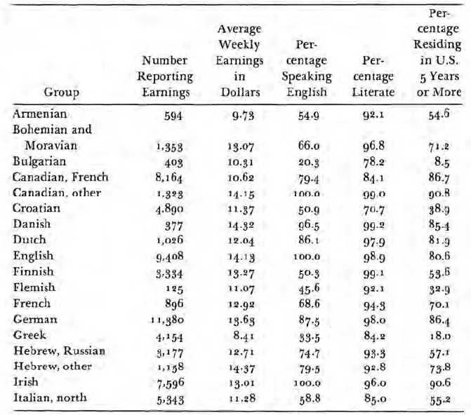
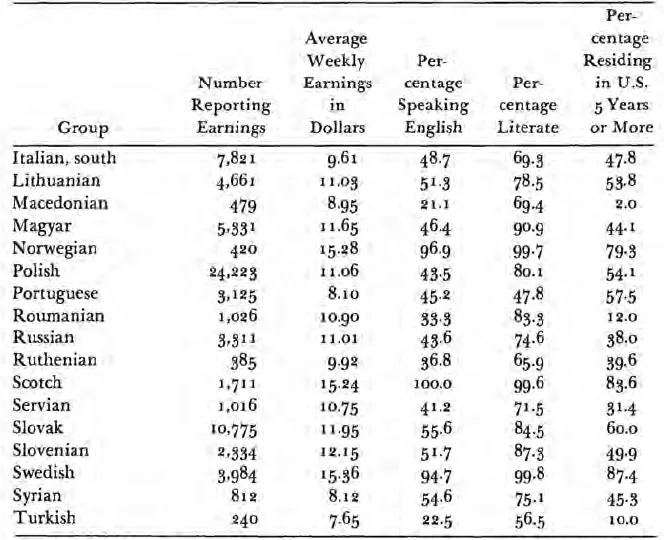
SOURCE. U. S. Immigration Commission, Report (Washington: Government Printing Office, 1911), I, pp. 367, 474, 439, 352, In this table, “literate” means able to read.

To test the hypothesis of skill differentials, a recent study employed the data shown in Table 5.2.⁹ Literacy and the ability to speak English serve as indexes of skill. The study found that the relation between earnings, ability to speak English, and literacy is best represented by the equation

Y = 2.55 + 0.0383E + 0.0796L

where Y is a group’s weekly average earnings in dollars, E is the percentage of a group speaking English, and L is the percentage of a group literate in any language. The equation can be interpreted as follows: holding the level of literacy constant, a 10-percentage-point increase in the proportion of a group speaking English was associated with an increase of about 38 cents per week in the group’s average earnings; holding the level of English-speaking constant, a 10-percentage-point increase in the proportion of a group literate was associated with an increase of almost 80 cents per week in the group’s average earnings. Each of these partial relations is statistically significant—could have been produced by pure chance less than one time in a hundred experiments—which means that the data are consistent with the hypothesis of skill differentials leading to earnings differentials. The overall relation statistically “explains” almost four fifths of the variance among the earnings of the groups; in statistical jargon, the equation provides a good “fit” for the data.

The Immigration Commission, which obtained the data shown in Table 5.2, also collected information from 41,933 native-born white employees in manufacturing and mining occupations to obtain a control group for its study of immigrants. The average earnings of these workers, all of whom spoke English and 98.2 percent of whom were literate, was $14.37 per week. To test the hypothesis that immigrants were the objects of ethnic discrimination, we use the equation relating skills to earnings among immigrants to predict the earnings of the native-born workers. If employers actually discriminated against immigrants, such a prediction would fall significantly below the actual earnings of the native-born workers. Remarkably, the prediction falls only 1 percent below the actual figure, a result that casts grave doubt on the notion that ethnic discrimination operated on a wide scale to the detriment of immigrant workers.¹⁰

This finding does not mean that no ethnic prejudice existed, and there is plenty of evidence that such prejudice did exist. But it is apparent that if some (discriminating) employers offered the immigrant a wage lower than the actual value of his labor services to the firm, another employer could increase his wealth by hiring that employee at a slightly higher wage. Of course, with many employers, each attempting to maximize wealth, competition for workers would soon force the wage up to a level at which it equalled the actual value of the worker’s labor services to the firm. Not every employer must be a wealth maximizer to obtain this result, however. In principle, just one would be enough, for it would pay him to outbid other (discriminating) employers for labor and to expand his business as long as he could continue to obtain workers at less than the going rate for equally skilled native-born workers. The evidence is quite convincing that at least some employers in the post-Civil War era strongly preferred wealth to the pleasures of discrimination. (Notice that our argument is just the reverse of the common belief that discrimination allows the employer to increase his wealth by “exploiting” his workers; this popular fallacy fails to take competition for labor into consideration.)¹¹

From these findings it is only a short step to an explanation of why each new immigrant group “came in at the bottom of the economic ladder.” It was partly because later groups were upon arrival less literate, which probably implies less skilled generally, than those having resided longer in the United States, and partly because they had less command of English, The ability to speak English was almost perfectly correlated with the duration of a group’s residence in America (Figure 5.2)—a good example of learning from experience, since few of these men ever received formal instruction in the English language. Over time the immigrants gained fluency in English and other skills, and in the process their earnings rose; those arriving later merely followed in the footsteps of those arriving earlier, and ethnic discrimination had little or no effect on the process. At any point in time, however, different groups occupied different positions on the ladder of skill acquisition, and hence correspondingly different positions on the earnings scale.

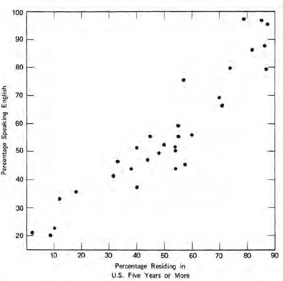
Figure 5.2 Relation between ability to speak English and length of residence in U. S., 31 non-English-speaking ethnic groups, 1909. Source: Table 5.2 above.

INEQUALITIES BETWEEN WHITES AND BLACKS

Inequalities between whites and blacks apparently existed in virtually all aspects of social and economic life throughout the post-Civil War era. Beyond this sweeping and obvious statement, however, very little can be said, for economic historians have just begun to study trends in racial inequalities during this period, and reliable findings have yet to appear. The absolute well-being of blacks certainly improved to some extent during the half century after the Civil War; the extremely low starting point, if nothing else, made some gains almost inevitable. Thousands of blacks migrated to regions of greater opportunity; a substantial majority learned to read and write; and many acquired land and other property—all of which worked to raise black incomes. Whether the rate of growth of black incomes exceeded the rate of growth of white incomes, however, remains open to conjecture. Given this dearth of knowledge, our discussion in this section can do little more than lay the groundwork for research that remains to be done.

Lacking income or earnings statistics, Gary Becker in his study of discrimination constructed an index of occupational standing for male blacks relative to male whites in nonfarm occupations in 1910. This index stood at 73 percent in the North and 67 percent in the South¹². A similar but more detailed and inclusive index constructed by Dale L. Hiestand stood at 78 percent for the entire nation in 1910.¹³ Unfortunately, however, the type of index constructed by Becker and Hiestand is biased upward as an indicator of relative earnings, for it assumes that the only difference between the races lay in their distribution among the various occupations—the index being less than unity because blacks were more concentrated in the lower-paying jobs. But a second source of differences in earnings, not captured by this index, is that within a particular job classification blacks typically earned less than whites. Moreover, blacks may have been more frequently unemployed. Clearly, indexes of relative occupational standing are open to serious objections, and in any event earlier observations are required before we can reach any conclusions about trends in the half century after the emancipation.

Any discussion of inequalities between whites and blacks in the post-Civil War era must take slavery as its point of departure. Under that system, slave owners had an interest in maintaining slaves at a level of well-being that would preserve their physical vitality, but beyond that level any outlays were wasted. Consequently, slaves existed at approximately the level of a physical subsistence income. Upon emancipation, blacks found themselves with few skills, without physical property, and concentrated in the devastated South. In the following half century they discovered that despite Constitutional amendments and civil-rights laws they had yet to attain full rights of citizenship. Lynch law took its toll in deaths and intimidation; many states devised ways of limiting black access to the polls; and white-dominated courts dealt out something less than equal justice. In effect, blacks labored under insecure civil liberties and uncertain private property rights, and this kind of “official” oppression constituted much more of an obstacle to their economic progress than discrimination against them in the market, though that also existed.

At any time in the past century, black earnings fall considerably below those of whites. This fact alone, however, implies nothing about racial discrimination in the labor market. To determine whether racial discrimination exists, we must be careful to compare workers identical in every respect except race, for even without racial discrimination, earnings differentials might exist because of differentials in age, sex, education, health, and other “productivity factors.” If earnings differentials remain after adjustment for productivity factors, the evidence is consistent with the hypothesis of purely racial discrimination.¹⁴ It is true, of course, that even if no discrimination exists in the labor market, earnings differentials could still be ascribed to discrimination if blacks are denied equal access to education or equal treatment under the law. Thus, discrimination may exist at two levels—in both the market and nonmarket sectors of resource allocation—and it is important to distinguish between them.

In the section above on “Immigrants and ‘Exploitation’,” we found that among immigrant groups in 1909, earnings and skills were closely related. We saw too that the earnings-skills relation gave an accurate prediction of the earnings of native-born white workers of comparable age, sex, and industrial affiliation. The Immigration Commission, which obtained the data used in our earlier tests, also collected comparable information from 6604 adult, native-born black males employed in mining and manufacturing industries in 1909. The workers in this sample earned an average of $10.66 per week. As a crude test of the racial discrimination hypothesis, we can use the earnings-skills relation presented in the previous section to predict the earnings of the black workers. If racial discrimination existed, the predicted earnings should significantly exceed actual earnings. In fact, the earnings predicted for this sample of black workers, all of whom spoke English and 76.4 percent of whom were literate, stands $1.80 above their actual earnings—a finding consistent with the hypothesis of racial discrimination, though a very crude finding to be sure.¹⁵

To say something more definite about the extent of labor market discrimination against black workers, we must obtain more detailed information on earnings and skills. Table 5.3 presents some crude industry data obtained from the report of the Immigration Commission. These data indicate no apparent relation between relative earnings and relative literacy or age, a finding that suggests that the earnings differentials may have been partly determined by discrimination. For the eight industries as a whole, however, black literacy does fall below white literacy in roughly the same proportion as earnings fall short. Still, these data are much too crude and too few to support any firm conclusions.

TABLE 5.3
EARNINGS, LITERACY, AND AGE OF BLACKS RELATIVE TO WHITES, ADULT MALE EMPLOYEES, 1909

Industry	Relative Mean Earnings	Relative Proportion Literate	Relative Mean Age
Agricultural implements and vehicles	0.86	0.93	1.09
Cigars and tobacco	0.62	0.80	1.04
Bituminous coal mining	0.86	0.78	1,03
Construction	0.74	0.75	0.92
Glass	0.72	0.86	1.09
Iron and steel	0.64	0.76	1.00
Iron ore mining	0.92	0.62	1.04
Meatpacking	0.93	0.95	0.98

SOURCE. Calculated from data in U. S. Immigration Commission, Report (Washington: Government Printing Office, 1911), XX, pp. 227–28, 270–71, 581, 1068–69.

The evidence considered in this section illustrates some of the difficulties in historical studies of racial discrimination. Perhaps, too, it can serve as a warning against drawing quick conclusions about a subject that engages strong emotions but remains little explored by scientific research. At present we can do little more than offer some conjectures for consideration in future studies. First, all existing evidence indicates more intense discrimination in the South than in the North. This fact suggests that a major determinant of the relative economic position of blacks has been their regional distribution. We need to know much more about what variables determined the rate and direction of black migrations, both interregionally and within the South. Second, differences between the economic progress of European immigrants and of blacks suggest three major hypotheses: that blacks began to accumulate skills from a much lower starting point than the immigrants; that blacks experienced greater discrimination than immigrants in the nonmarket sector, especially in obtaining education and equal treatment under the law; or that ethnic prejudice against blacks in the labor market was more intense and widespread than that against immigrants. Combinations of these hypotheses are of course possible. Third, discrimination against blacks in the market often depended on discrimination in the nonmarket sector, as, for example, when Southern white employers who strongly preferred wealth to discrimination, and would have bid up black wages, were illegally intimidated by fellow whites intent on keeping the black “in his place.” We need to know much more about the relation between the market and the nonmarket varieties of discrimination and about the enforcement techniques employed within the white community to maintain effective discrimination.

WAS PROGRESS WORTH ITS PRICE?

A comparison of the American economy in 1865 with the economy in 1914 points up a variety of changes. On the eve of the Great War Americans consumed about three times more economic goods per capita than they had a half century earlier. They lived longer and healthier lives and spent less time at work and more at recreation. They were better housed and educated, traveled more, read more, and were better informed about their own and other countries. All of this we customarily call Progress.

Against the gains of economic growth, however, must be set the costs of realizing the gains. Economic growth was an inherently disruptive process, and because certainty itself is an economic good, unanticipated disruptions constituted one of the costs of growth. Business depressions erratically punctuated the course of growth, leaving workers without jobs and employers with losses, but in an unregulated market economy such fluctuations were both unavoidable and unpredictable (Table 5.4).

TABLE 5.4
ESTIMATED PERCENTAGE OF LABOR FORCE UNEMPLOYED IN SELECTED DEPRESSION YEARS

Year	Percentage Unemployed
1876	12–14
1885	6–8
1894	18
1908	8

SOURCE. Stanley Lebergott, Manpower in Economic Growth (New York: McGraw-Hill, 1964), pp. 187, 512, 522.

Though inventions led to increased efficiency in production, they often meant bankruptcy for those employing older processes. David A. Wells, despite his pervasive optimism, was perceptive enough to recognize that “nothing marks more clearly the rate of material progress than the rapidity with which that which is old and has been considered wealth is destroyed by the results of new inventions and discoveries.”¹⁶ Though migration allowed young people to obtain higher incomes, it often left their parents lonely and unhappy in the old home. Though the settlement of fertile Western lands provided cheaper food for urban dwellers, it often meant ruin for Eastern farmers. And similar contrasts might be recited at great length. We could say that people did adjust; ultimately everyone was better off. But such an interpretation is incomplete and ignores the costs imposed on people by the disruptive transformations that inevitably accompanied economic growth.

The inescapable fact is that economic growth hurt many people. Some recovered their losses, but others did not. Economic growth meant Progress from a social point of view because it created more wealth than it destroyed, but the distribution of the gains and losses was quite unequal. If we are interested in individual welfare, the answer to the question “Was progress worth its price?” must necessarily be that for some it was, and for others it was not. It will hardly do to say that individuals “freely chose to have economic growth,” because growth was a social process; the actions of a single individual simply did not matter one way or the other. An individual could determine his own program of saving and investment, but he could neither foresee nor control the future development of the market system. He could not know that the investments made in such hopeful expectations and based on the most reliable available information were often destined to become reductions in his wealth.

American society encouraged economic growth by guaranteeing individuals secure private property rights and free access to markets, but the specification of property rights did not permit all economic actions and their effects to be determined through free contracting. In the absence of all-embracing rights of contract—an impossibility in any event—many external or “spillover” effects were inevitable, some of them beneficial but others quite harmful. The Supreme Court clearly recognized the problem in deciding the case of Coppage v. Kansas (1915):

No doubt, wherever the right of private property exists, there must and will be inequalities of fortune; and thus it naturally happens that parties negotiating about a contract are not equally unhampered by circumstances. . . . Since it is self-evident that unless all things are held in common, some persons must have more property than others, it is from the nature of things impossible to uphold freedom of contract and the right to private property without at the same time recognizing as legitimate those inequalities of fortune that are the necessary result of the exercise of those rights.¹⁷

By not holding people liable for all the effects of all their actions, American society widened the scope of free individual actions, but at the same time it forfeited the kind of security and order that can exist in a stationary economy. In a free market economy the race was to the swift—and, of course, to the lucky, for even the swift sometimes ran in the wrong direction.

1 Harvey S. Perloff, et al., Regions, Resources, and Economic Growth (Baltimore: Johns Hopkins, 1960), p. 579. The simple coefficient of correlation between wages per worker and capital pet worker is 0.63, a level that could have been produced by pure chance less than one time in a thousand experiments.

2 Actually, resource transfer is attractive only when the present value of the expected gains obtainable by the transfer exceeds the costs of the transfer: the migration of resources should be considered in the same terms as any other investment. In the present discussion we are abstracting from the costs of the transfer.

3 C. Vann Woodward, Origins of the New South, 1877-1913 (n. p.: Louisiana State University, 1951), p. 473.

4 Richard A. Easterlin, “Regional Income Trends, 1840–1950,” in Seymour E. Harris, Ed., American Economic History (New York: McGraw-Hill, 1961). p. 527.

5 Stanley L. Engerman, “The Economic Impact of the Civil War,” Explorations in Entrepreneurial History, III (Spring/Summer 1966), 194, n. 20.

6 In particular, the National Banking Act, passed during the Civil War, did much to retard Southern recovery. See Richard Sylla, “Federal Policy, Banking Market Structure, and Capital Mobilization in the United States, 1863–1913,” Journal of Economic History, XXIX (Dec. 1969).

7 Jacob Riis, How the Other Half Lives (New York: Charles Scribner’s Sons, 1890), pp. 123–24, 136.

8 Oscar Handlin, The Uprooted (Boston: Little, Brown and Company, 1952), p. 195.

9 Robert Higgs, “Race, Skills, and Earnings: American Immigrants in 1909,” Journal of Economic History, XXXI (June 1971). This paper contains an assessment of the data shown in Table 5.2; it also presents the technical features of the statistical results summarized below and a more detailed discussion of the problems examined in this section.

10 The predicted earnings figure is 2.55 + 0.0383 (100.0) + 0.0796 (98.2) = 14.20.

11 For a complete discussion of the theory summarized in this paragraph, see Gary S. Becker, The Economics of Discrimination (Chicago: University of Chicago, 1957), especially pp. 35–37.

12Ibid., p. 113.

13 Dale L. Hiestand, “The Changing Position of Negro Workers,” in John F. Kain, Ed., Race and Poverty (Englewood Cliffs, N. J.: Prentice-Hall, 1969), p. 72.

14 For an example of a study that makes such adjustments, employing data for 1960, see James D. Gwartney, “Discrimination and Income Differentials,” American Economic Review, LX (June 1970).

15 The predicted earnings figure is 2.55 + 0.0383 (100.0) + 0.0796 (76.4) = 12.46.

16 David A. Wells, Recent Economic Changes (New York: Appleton, 1889), p. 31.

17 Cited in John R. Commons, Legal Foundations of Capitalism (New York: Macmillan, 1924), p. 291.