Appendix: A Mathematical Model of Free Banking

The specification of the model takes the following forms:
Implicitly,

MD = MD(P;k,y)

MS = MS(P;S,k,P_s,y)

Y= Y(P;y)

Explicitly,

MD = aP + by + ck(1)

MS = eS + fk − gP_s− hP − jy(2)

Y= Py(3)

where

MD = the nominal demand for money

MS = the nominal supply of money

k = the fraction of income consumers desire to hold as money

y = real national income (output)

S = the specie reserves of banks

P = the price level

P_s = the real unit cost of specie

Y = nominal national income

It is assumed that a > , b > , c > , e > , f > , g > , h > , j > , l > k > . In equilibrium MS = MD = M. Taking M, P, and Y as the endogenous variables of the system, this becomes:

M − aP = by + ck (1a)

M + hP = eS + fk − gP_s − jy(2a)

Y − Py = (3a)

Setting this up in the matrix form Ax = d, one has the following:

solving for the determinant |A| = (h + a)>. Thus, there exists a unique and nontrivial solution to the system. Utilizing Cramer’s Rule, one can solve for M, P, and Y, the equilibrium values of M, P, and Y.

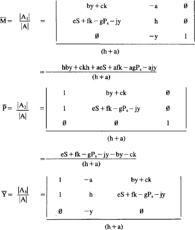
To determine the effects of parametric changes, one may take the partial derivative of each M, P, and Y with respect to k, y, S, and P_s.

If k changes,

To maintain monetary equilibrium,

Therefore,

and

To summarize,

An increase in k increases both the demand for money and the supply of money. The price level and nominal income do not change.

If y changes,

To maintain equilibrium, one must take account of shifts of the curves, that is,

As well as movements along the curves, that is,

Substituting,

Since

then

Since

then

Following George Selgin (1988a, 98–101; 1990, 272), if one assumes that aggregate demand is unit elastic, ∂Y/∂P + ∂Y/∂y = , and since ∂Y/∂P = , then ∂Y/∂y = . This means that P(h + a) = y(j + b), which is to say that the price level times its effects on MS and MD equals real output times its effects on MS and MD. One may note that if aggregate demand were elastic, then ∂Y/∂y>, and if aggregate demand were inelastic, then ∂Y/∂y< . To summarize,

A pervasive increase in productivity will drive production costs and the price level down. Nominal money demand rises, while the nominal money supply falls. Nominal money holdings remain the same, as does nominal income.

If S changes, then

If there occurs an unanticipated increase in the supply of specie (monetary gold), then the money stock, the price level, and nominal national income all rise. It is more likely, however, that such a change in the production of specie would be preceded by an increase in the demand for same. In other words, first k_o rises and k_i falls. This constitutes a redemption run.

For changes in k_i,

For changes in the real cost of specie (P_s),

The relative demand for specie rises, driving up its price (P_s). The desired ratio of outside money to inside money, k_o/k_i, also rises. The inside money supply falls by a larger proportional amount than the outside money supply rises. The price level and nominal income decline. Subsequently, the supply of specie increases. This increases both the outside and inside money supplies, the price level, and nominal income.

A currency run occurs when consumers choose to liquidate part or all of their deposit accounts in order to acquire currency. Currency runs pose a deflationary threat to central banking systems, because all currency runs are also redemption runs. This follows from the facts that (1) there is a single monopoly issuer of currency, and (2) in such a system, the legal tender currency serves both as currency for the public and as part of the reserves of commercial banks.

Under central banking,

MS = C + DD and MB = C + R,

where

MS = the money supply

C = currency held by the public

DD = demand deposits

MB = the monetary base

R = bank reserves (vault cash plus deposits with the central bank)

If the statutory reserve ratio is RR, then . Substituting the expression for DD back into the earlier expression for MS, . Since R = MB–C, then

This last is clearly negative as long as RR < 1, that is, as long as there is fractional reserve banking. Also, | 1 - 1/RR | > 1 if RR <.5, which is very likely. For example, if the legal tender reserve ratio is 0.1 and consumers exchange $1 million in deposit credits for $1 million in currency, for any given monetary base, the net effect on the money supply will be a decrease of $9 million.

Under free banking,

MS = N + DD and MB = S

where

MS = the inside money supply

N = privately issued banknotes

DD = demand deposits

MB = the monetary base

S = banks’ specie reserves

If OR_N is the optimal reserve ratio for notes, OR_DD is the optimal reserve ratio for demand deposits, S_N the specie reserves for notes, and S_DD the specie reserves for demand deposits, then

or

If all free banks exhibit the same optimal reserve ratios for each deposits and notes, then OR_N = OR_DD = OR.

Keeping in mind that specie reserves can be used to redeem either notes or deposits, the above expression for the money supply may be transformed such that

Thus,

An increased relative demand for currency (versus deposits) has no net effect on the money supply under free banking. It is not necessary for a currency run to become a redemption run, as is the case under central banking.