Appendix A: Marginal Physical and Marginal Value Product. 500

For purposes of simplification, we have described marginal value product (MVP) as equal to marginal physical product (MPP) times price. Since we have seen that a factor must be used in the region of declining MPP, and since an increased supply of a factor leads to a fall in price, the conclusion of the analysis was that every factor works in an area where increased supply leads to a decline in MVP, and hence in DMVP. The assumption made in the first sentence, however, is not strictly correct.

Let us, then, find out what is the multiple of MPP that will yield an MVP. MVP is equal to an increase in revenue acquired from the addition of a unit, or lost from the loss of a unit, of a factor. MVP will then equal the difference in revenue from one position to another, i.e., the change in position resulting from an increase or decrease of a unit of a factor. Then, MVP equalsR₂ – R₁, where R is the gross revenue from the sale of a product, and a higher subscript signifies that more of a factor has been used in production. The MPP of this increase in a factor is P₂ – P₁, where P is the quantity of product produced, a higher subscript again meaning that more of a factor has been used.

So: MVP = R₂ – R₁ by definition.

MPP = P₂ – P₁ by definition.

Revenue is acquired by sale of the product; therefore, for any given point on the demand curve, total revenue equals the quantity produced and sold, multiplied by the price of the product.

Therefore, R = P · p, where p is the price of the product.

So: R₂ = P₂ · p₂

R₁ = P₁ · p₁

Now, since the factors are economic goods, any increase in the use of a factor, other factors remaining constant, must increase the quantity produced. It would obviously be pointless for an entrepreneur to employ more factors which would not increase the product. Therefore, P₂ > P₁.

On the other hand, the price of the product falls as the supply increases, so that:

p₂ < p₁

Now, we are trying to find out what multiplied by MPP yields MVP. This unknown will be equal to:

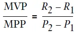
This may be called the marginal revenue, which is the change in revenue divided by the change in output.

It is obvious that this figure. which we may call MR, will not equal either p₂ or p₁, or any average of the two. Simple multiplication of the denominator by either of the p's or both will reveal that this does not amount to the numerator. What is the relation between MR and price?

A price is the average revenue, i.e., it equals the total revenue divided by the quantity produced and sold. In short,

But above, in the discussion of marginal and average product, we saw the mathematical relationship between “average” and “marginal,” and this holds for revenue as well as for productivity: namely, that in the range where the average is increasing, marginal is greater than average; in the range where average is decreasing, marginal is less than average. But we have established early in this book that the demand curve—i.e., the price, or average revenue curve—is always falling as the quantity increases. Therefore, the marginal revenue curve is falling also and is always below average revenue, or price. Let us, however, cement the proof by demonstrating that, for any two positions, p₂ is greater than MR. Since p₂ is smaller than p₁, as price falls when supply increases, the proposition that MR is less than both prices will be proved.

First, we know that p₂ < p₁, which means that

Now, we may take point one as the starting point and then consider the change to point two, so that:

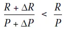
thus translating into the same symbols we used in the productivity proof above. Now this means that

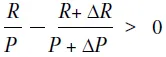
Combining the two fractions, and then multiplying across, we get

RΔP – PΔR > 0

or

RΔP > PΔR,

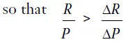
(We have here proved that MR is less than p₁, the higher of the two prices.)

Now this means that there is some unknown, constant positive fraction l/k which, multiplied by the larger, will yield the smaller ratio (MR) in the last inequality. Thus,

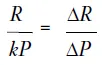
Now, by algebra,

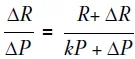
and since k is a positive number,

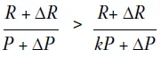
But this establishes that

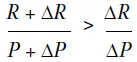
i.e., that MR is less than p₂. Q.E.D.

Hence, when we consider that, strictly, MR, and not price, should be multiplied by MPP to arrive at MVP, we find that our conclusion—that production always takes place in the zone of a falling MVP curve—is strengthened rather than weakened. MVP falls even more rapidly in relation to MPP than we had been supposing. Furthermore, our analysis is not greatly modified, because no new basic determinants—beyond MPP and prices set by the consumer demand curve—have been introduced in our corrective analysis. In view of all this, we may continue to treat MVP as equaling MPP times price as a legitimate, simplified approximation to the actual result.³⁴